7  ClassificationⅡ

7.1 Summary

KEY ASPECT	DETAILS
Classification Techniques	- FCNN mapping - Pre-processing importance - Data normalization
OBIA	- SLIC algorithm for superpixels - Spatial distance and color balance
Sub-pixel Analysis	- Land cover proportions per pixel - Reflectance formula application
Accuracy Assessment	- Confusion matrices - Producer’s, user’s, and overall accuracy - Spatial cross-validation

7.1.1 Dynamic World’s Semi-supervised Approach

• Divides the globe into regions and biomes.

• Uses stratified sampling based on NASA MCD12Q1 land cover data and others.

• Training involved labeling ~4,000 image tiles by experts and 20,000 by non-experts.

7.1.2 Classification Techniques

• FCNN (Fully Convolutional Neural Network): Learns the mapping from estimated probabilities back to input reflectances.

• Pre-processing: Important for data quality, including cloud masking and normalization of data.

• Normalization: Log-transform raw reflectance values and remap to a sigmoid function to equalize highly reflective surfaces.

7.1.3 Object-Based Image Analysis (OBIA)

• Uses the SLIC algorithm for superpixel generation, focusing on the balance between spatial distance and color homogeneity.

Bears in right picture are objected based, and similar pixels are clustered as superpixels

Source: Darshite Jain

• Formula for balancing physical distance and color: S (initial point distance), m (compactness), and considerations for Euclidean distance. \[ D = \sqrt{{\left(\frac{d_{\text{color}}}{m}\right)^2 }} + \left(\frac{d_{\text{space}}}{S}\right) \]

7.1.4 Sub-pixel Analysis

• Spectral Mixture Analysis (SMA): Determines the proportion of landcover per pixel. For example, it shows how many percent of urban area, and how many percent of vegetation, and how many percent of water.

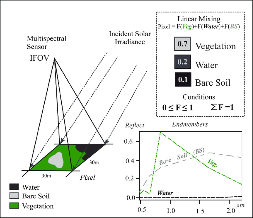
Source: Paul, Machado & Small (2013)

• Reflectance represented by the sum of endmembers weighted by their fraction: \[ p_{\lambda} = \sum_{i=1}^{n} (p_{i\lambda} * f_i) + e_{\lambda} \]

7.1.5 Accuracy Assessment

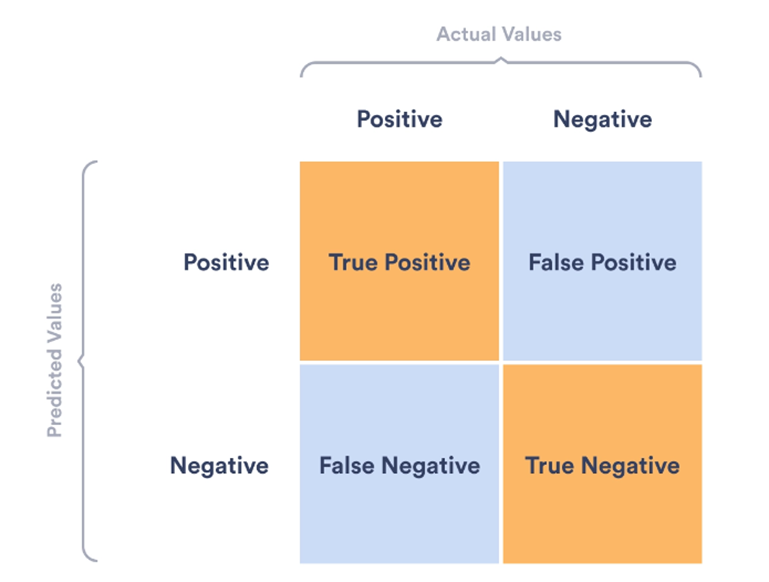
Confusion Matrix Source: bloginformation.co.kr

• Producer’s Accuracy (PA): Measures the match between classified data and ground truth, showing how accurately the model identifies classes \[ TP/TP+FN \]

• User’s Accuracy (UA): Indicates the reliability of the classification for users, reflecting the likelihood that a classified instance actually represents its assigned class in reality. \[ TP/TP+FP \]

• Overall Accuracy (OA): Provides a general measure of the model’s performance, representing the total proportion of correctly classified instances. \[ TP+TN/TP+FP+FN+TN \]

  To enhance model accuracy assessment, spatial cross-validation addresses spatial autocorrelation by ensuring training and testing datasets are spatially independent.

  

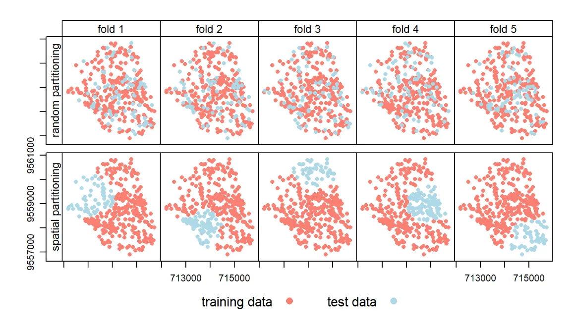
  Illustration of default cross-validation vs. spatial cross-validation. Source: Lovelace, et al (2021)

  The Kappa Coefficient measures classification accuracy against chance, with values between -1 and 1. The balance between recall and precision is evaluated using the F1-Score, which helps navigate the challenges of false positives and negatives. Additionally, the Receiver Operating Characteristic (ROC) Curve and the Area Under the Curve (AUC) assess model performance by focusing on true positive rates and minimizing false positives. These techniques collectively offer a detailed framework for a more accurate and comprehensive evaluation of classification models.

\[ F_1\text{-score} = 2 \times \frac{\text{Precision} \times \text{Recall}}{\text{Precision} + \text{Recall}} = \frac{2TP}{2TP + FP + FN} \]

7.2 Applications

7.2.1 Sub-Pixel Analysis for Dynamic Flood Monitoring

Innovative Approach to Flood Monitoring

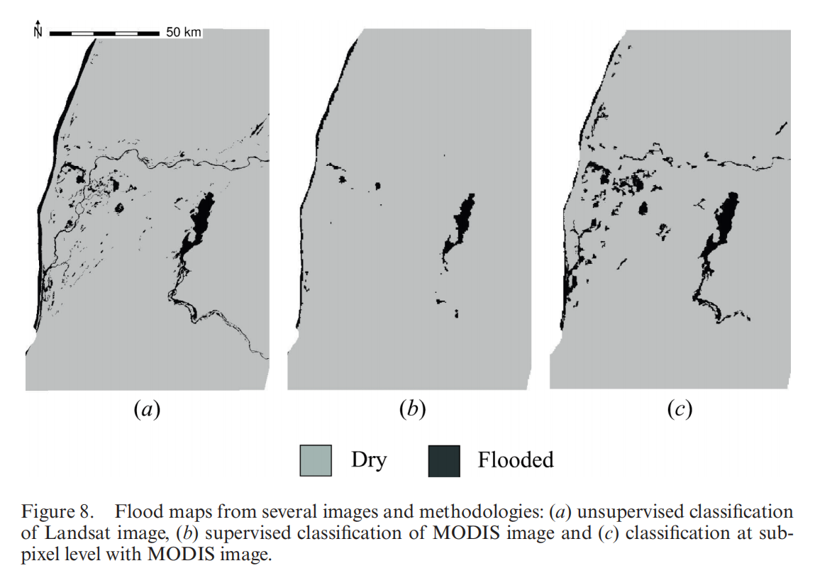
Giraldo Osorio and García Galiano’s (2012) research uses sub-pixel analysis (SA) method to accurately identify and monitor flood extents using optical images with moderate spatial resolution. This approach overcomes the limitations of traditional classification methods by incorporating primary topographic attributes derived from DEMs, facilitating more precise flood delineation even in areas where detailed spatial data are scarce.

Methodology and Implementation

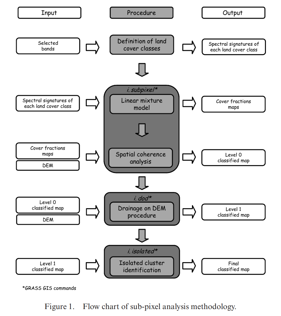
The SA method begins with the resolution of the Linear Mixture Model (LMM) to calculate land cover fractions within coarse pixels. This process is informed by the underlying DEM, aiming to prioritize the mapping of flooded areas in lower terrain sections. The method’s efficacy is further enhanced through spatial analysis techniques that account for the distribution of water classes within the pixel and its surrounding environment.

Practical Outcomes and Flood Mapping Enhancement

Applied to the monitoring of flood events in the lower Senegal River Valley, this methodology showcased a remarkable improvement in mapping flood extents compared to conventional classification techniques. The study achieved an approximate 80% accuracy in correctly mapping flooded areas across various regions, significantly outperforming traditional supervised classification methods.

7.2.2 Cross Validation VS Spatial Cross-validation (Karasiak et al. 2021)

In the processing and analysis of remote sensing data, accuracy assessment is a key indicator for measuring the quality of classification results. This case study focuses on using Sentinel-2 data to classify forest cover types (coniferous and broadleaf forests) and explores the impact of spatial cross-validation (SCV) and non-spatial cross-validation methods on the assessment of classification accuracy.

Experimental Design

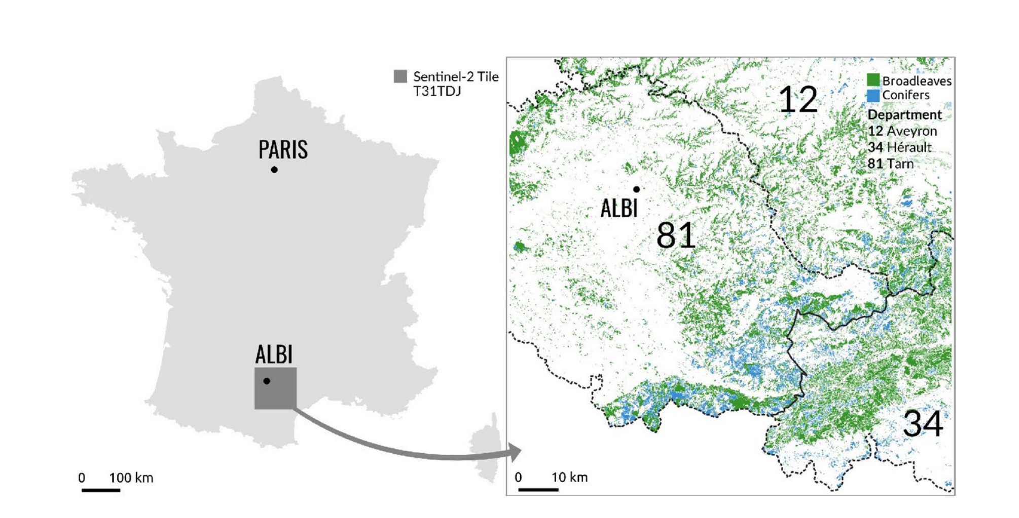
Location of the 31TDJ Sentinel-2 tile in the south of France

• Data and Preprocessing: Sentinel-2 imagery data was selected for classifying coniferous and broadleaf forests in specific areas. Data preprocessing steps included cloud removal and atmospheric correction to ensure data quality.

• Classification Method: The random forest algorithm was used for classifying forest types, considering its effectiveness in handling high-dimensional data and robustness to noise.

• Accuracy Assessment Method: Both non-spatial cross-validation and spatial cross-validation methods were applied to assess the accuracy and generalization ability of the classification model.

Results and Analysis

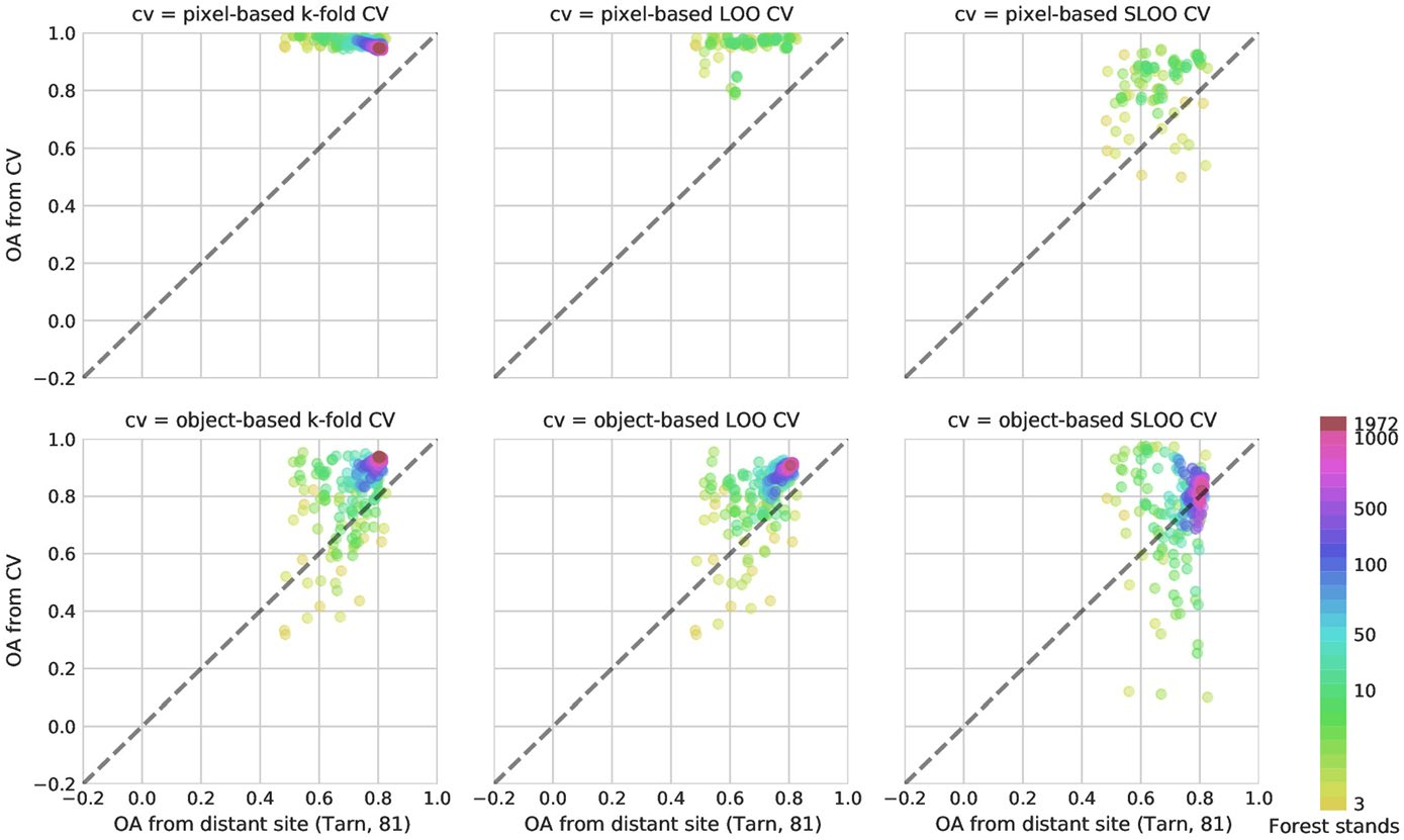
Comparison between the predictive performances obtained with spatial and non-spatial

cross-validation

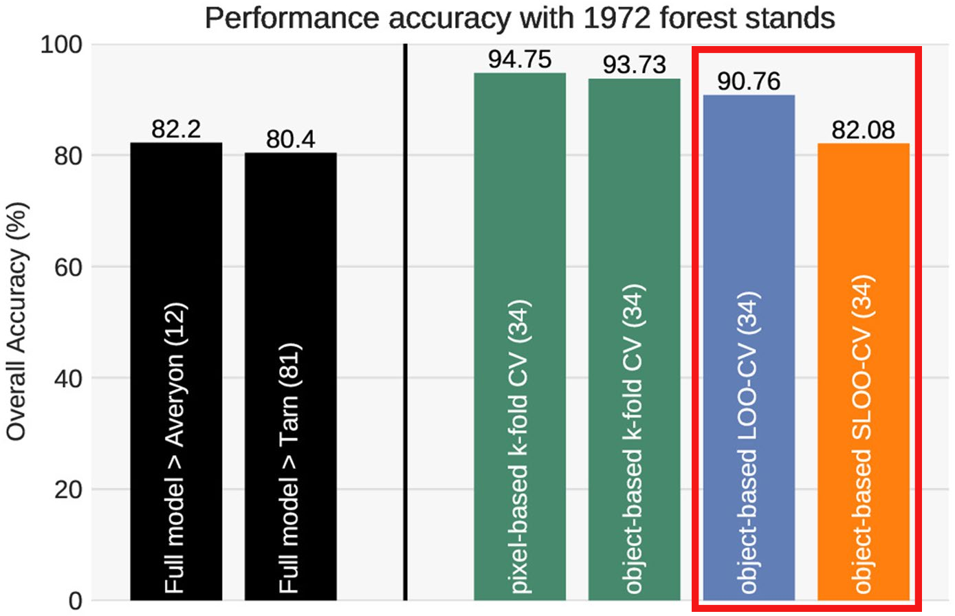
• Accuracy Comparison: The results showed that the overall accuracy assessment of the model using SCV was lower than that obtained by non-spatial cross-validation methods, but it more realistically reflected the model’s generalization ability.

• Validation of Generalization Ability: By applying the trained model to independent testing areas, the model assessed by SCV demonstrated better generalization ability, i.e., higher prediction accuracy on unseen data.

Why SCV Can More Accurately Assess Model Generalization Ability

• Spatial Autocorrelation: Pixels in remote sensing data often exhibit spatial autocorrelation, meaning physically neighboring pixels are more similar in attributes. Non-spatial cross-validation ignores this, potentially leading to an overestimation of the model’s generalization ability.

• Spatially Independent Test Set: SCV ensures that samples in the test set are spatially independent from the training set samples, effectively avoiding overly optimistic accuracy assessment due to spatial autocorrelation.

• Reducing the Risk of Overfitting: SCV reduces the model’s overfitting to specific data distributions, thereby more truthfully reflecting the model’s predictive ability on unknown data.

7.3 Reflection

The intricate process of spatial segmentation required for SCV has brought to light the challenging balance between achieving rigorous model validation and the necessity of managing computational resources effectively. This balance is particularly crucial when processing extensive datasets, where the computational demands can escalate quickly.

Delving into sub-pixel analysis to monitor flood extents further expanded my appreciation for the innovative methodologies that navigate the computational hurdles of remote sensing data analysis. It showcased how advanced techniques could provide more accurate environmental monitoring by accounting for spatial autocorrelation—acknowledging that data points in proximity are often more alike than those further apart, which is a vital consideration for enhancing model accuracy.

These studies have profoundly influenced my approach to remote sensing data, particularly in recognizing the importance of spatial patterns and their impact on analytical outcomes. The week has been a pivotal reminder of the necessity to integrate a thorough understanding of the spatial attributes of data with sophisticated analysis techniques.

7.4 References

Karasiak, N. et al. (2021) ‘Spatial dependence between training and test sets: another pitfall of classification accuracy assessment in remote sensing’, Machine Learning, 111(7), pp. 2715–2740.

Lovelace, R., Nowosad, J. & Muenchow, J. (2021). ‘Statistical Learning: Spatial CV’, in Geocomputation with R.

Paul, R., Machado, P. & Small, C. (2013). Identifying multi-decadal changes of the Sao Paulo urban agglomeration with mixed remote sensing techniques: spectral mixture analysis and night lights.